This is Part 2 of a series on understanding your own EEG, using accessible tools to dig into your own data. Please check out Part 1: Reading Your Own QEEG: Neuroguide & SigViewer, for an overview on looking at signals and flat QEEG “maps”.  You might also want to check out my article on Biohacking With EEG Phenotypes, which can help orient you to this landscape of EEG patterns.

What is LORETA?

LORETA (Low Resolution Electromagnetic Tomography) is an advanced neuroimaging technique used to analyze and visualize electrical activity in the brain. This can get pretty complex, as a number of sources can be generating local current densities in different parts of the brain, coming from distributed sources.

The Inverse Problem: EEG Source Localization From Surface QEEG Brain Maps 

The difficulty of “seeing” individual sources of brain activity is due to the EEG mixing and spreading as it is generated – you are making millions of point-sources of electricity deep inside your brain, and at the scalp these become mixed together under each of the electrodes that are used to record at the scalp. Thus, solving the EEG inverse problem involves estimating local and distant contributions at each electrode, and developing a signature for each one using this distributed source model.

Developed by Roberto Pascual-Marqui and colleagues to solve this difficulty, LORETA considers the instantaneous EEG at each electrode and the lagged EEG at each electrode, and unmixes the sources to estimate location of generators. This offers several key advantages in EEG analysis:

1. 3D Localization: Unlike traditional EEG which provides a 2D representation of brain activity on the scalp, LORETA uses sophisticated algorithms to estimate the source of electrical activity within the 3D structure of the brain.
2. Improved Spatial Resolution: While EEG has excellent temporal resolution, its spatial resolution is limited. LORETA significantly enhances spatial resolution, allowing for more precise localization of brain activity.
3. Deep Brain Structures: LORETA can estimate activity in deeper brain structures, not just cortical surface activity.
4. Standardized Analysis: LORETA uses a standardized head model and electrode positions, allowing for consistent analysis across subjects and studies.
5. Multiple Frequency Bands: It allows for the analysis of brain activity across different frequency bands (delta, theta, alpha, beta, gamma), providing a comprehensive view of brain function.

LORETA has evolved over time, with newer versions including sLORETA (standardized LORETA) and eLORETA (exact LORETA), each offering improvements in accuracy and resolution. By transforming traditional EEG data into 3D visualizations, LORETA provides researchers and clinicians with a tool for understanding brain function in specific brain regions, and adds a brain imaging perspective in 2D and 3D, and for both cortical and subcortical sources.

You can use this free tool to understand more about areas of your brain. This article won’t be a full guided tour through LORETA, but by the end of this post you should be able to take text exports of your own EEG data, and visualize brain electrical activity for features in your QEEG that you are interested in learning more about.

So what is LORETA doing?  Essentially it is “unmixing” the contributions at the scalp EEG level from multiple cortical EEG sources, and projecting the source locations onto a mathematical model of how EEG is generated throughout the human head,  The LOR in LORETA stands for “low resolution” because the spatial solutions are still not as precise as fMRI, especially using the standard 19 electrode “grid” that is used for most classic EEG, including sleep studies, seizure monitoring, QEEG brain mapping, and a great deal of research over the past 100 years. Dr. Pasqual-Marquis has published multiple papers showing that the sources estimated in the EEG match those of other sources shown in fMRI and MEG, even while losing resolution at low electrode density. Also, LORETA can be done in a “high density” EEG grid. As the number of EEG electrodes increases, the resolution of tool improves. Dr. Pasqual-Marquis has presented comparison data at conferences showing that at 70 electrodes sLORETA becomes as spatially accurate as fMRI at estimating small localized sources of activity.

Current use of LORETA is broad and deep, and used in research and clinical contexts. The LORETA source estimation tools are built into several workhorse tools in the neurofeedback space, including QEEG database analysis tools and real-time LORETA neurofeedback tools.

We will mostly use LORETA as the sLORETA version in this tutorial, to work out the “EEG inverse problem” for any QEEG features we want to explore with this EEG source analysis method. This uses a free version of LORETA tools to get you doing your first analyses and visualization of data, but we will not get to more advanced LORETA topics here. See later on in the article for some of those topics. LORETA has really good demo tutorials to help you learn most of those processes.

Introduction: EEG Source Imaging to Explore Your QEEG Results

After reviewing your flat QEEG maps and Continuous Performance Test (CPT) results, you may have identified specific patterns of EEG activity that warrant further investigation. The process of QEEG has an implicit statistical analysis, as it is generating population-difference maps, but it is important that you first look at your raw EEG and know what sources of noise you want to avoid including in a LORETA (and sLORETA) analysis – artifact will get “solved” into false EEG sources, so a LORETA analysis requires fairly clean EEG for valid source reconstruction.

If you have not read Part 1, on understanding your own QEEG, check that out to orient yourself to using raw EEG trace data and Neuroguide maps (a standard commercial analysis tool and database used in QEEG and neurofeedback).

This guide will walk you through the process of using LORETA to create detailed 3D visualizations of features in your QEEG, helping you display EEG generators, or brain sources, derived from scalp EEG using advanced analysis techniques.

Downloading and Installing sLORETA: Visualize EEG Brain Activity 

Before we begin the analysis, let’s ensure you have LORETA properly installed. We will refer to the overall process and software as “LORETA” but will be using the more advanced sLORETA solutions. The sLORETA method is default the current version of LORETA software.

Request Download and get Password

1. Access the LORETA download page: https://www.uzh.ch/keyinst/loreta.htm
2. Select “LORETA-Key Alpha Software Download”
3. Agree to the license agreement
4. You’ll receive a message to send a blank email key.loreta@gmail.com for the download link and password. The password will be mailed back to you.

LORETA Installation steps:

1. Run the downloaded .exe file
2. Save the program to your preferred location
3. The main folder will be named “LoretaKey” with auto-populated files and resources
4. Use the Loreta Desktop Shortcut creator within the folder to create a shortcut with administrator privileges

Once you run the application and agree to the license, you will be met with a functioning instance of LORETA! Note, if your LORETA application icon says sLORETA, it may be an older 32-bit version from 2008 instead of the current version.  This tutorial will still work, but some of the buttons and options will be moved around.

Select Electrical Sources for the Inverse Problem: Use QEEG Brain Map & CPT

Before diving into the LORETA analysis, take a few minutes examine your QEEG and CPT results for features and phenotypes you want to explore further:

1. Review your signals in SigViewer plus flat QEEG maps across different frequency bands (delta, theta, alpha, beta).
   • Make sure to look at two montages, i.e. both Linked Ears and Laplacian (Current Source Density) to get a sense of which areas to investigate
   • Peak Brain uses Linked and Lap as the two standard montage. Linked is a standard montage, but any other montage such as Average or Global may be used in comparison. Always look at your QEEG in two montages – they display different spatial information in QEEG “flat” maps.
2. Note any areas showing significant deviations from the norm (high or low activity on the z-score “Bell curve” scale)
3. Correlate these findings with your CPT results and goals for of difficulties with your performance.
4. Identify specific frequencies and brain regions you want to explore further with source imaging

Raw EEG (Linked Ears, Eyes Closed)

QEEG (Laplacian, Eyes Closed)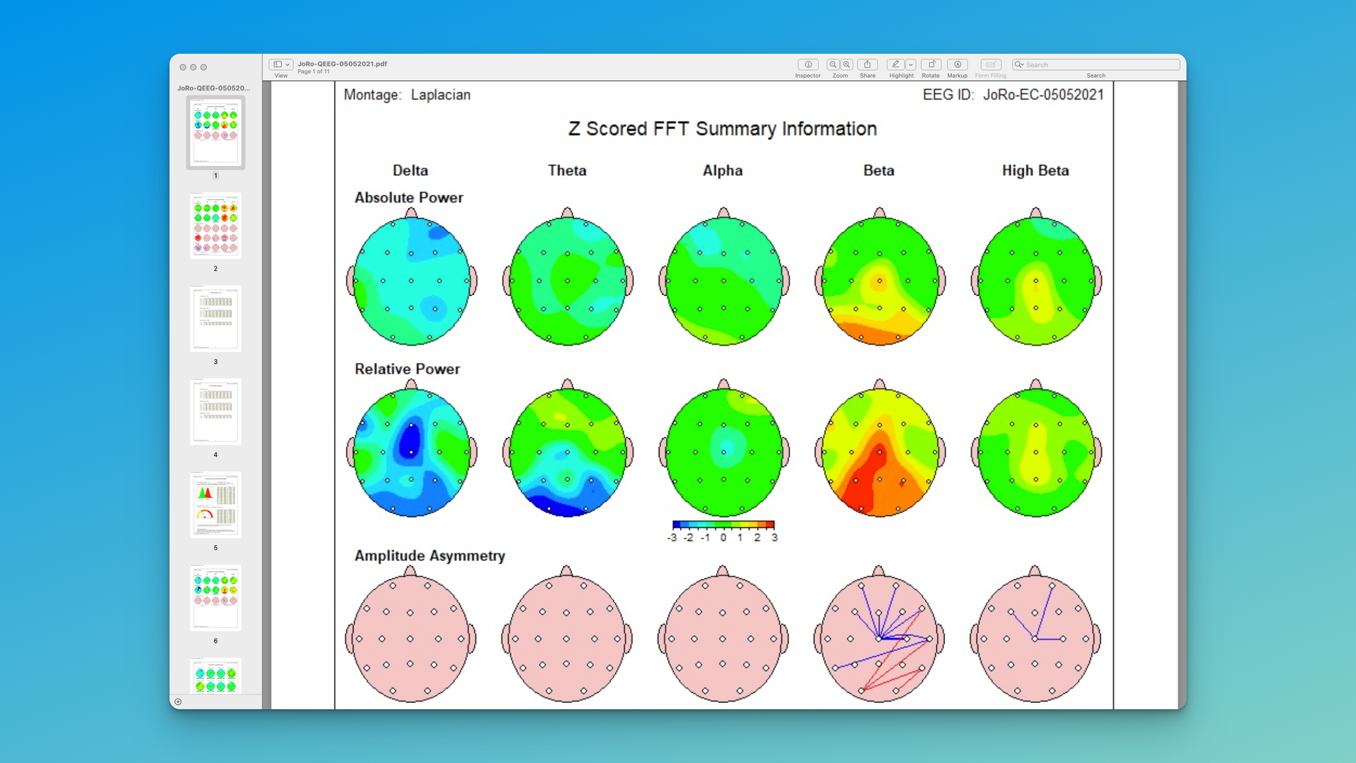

QEEG (Linked Ears, Eyes Closed)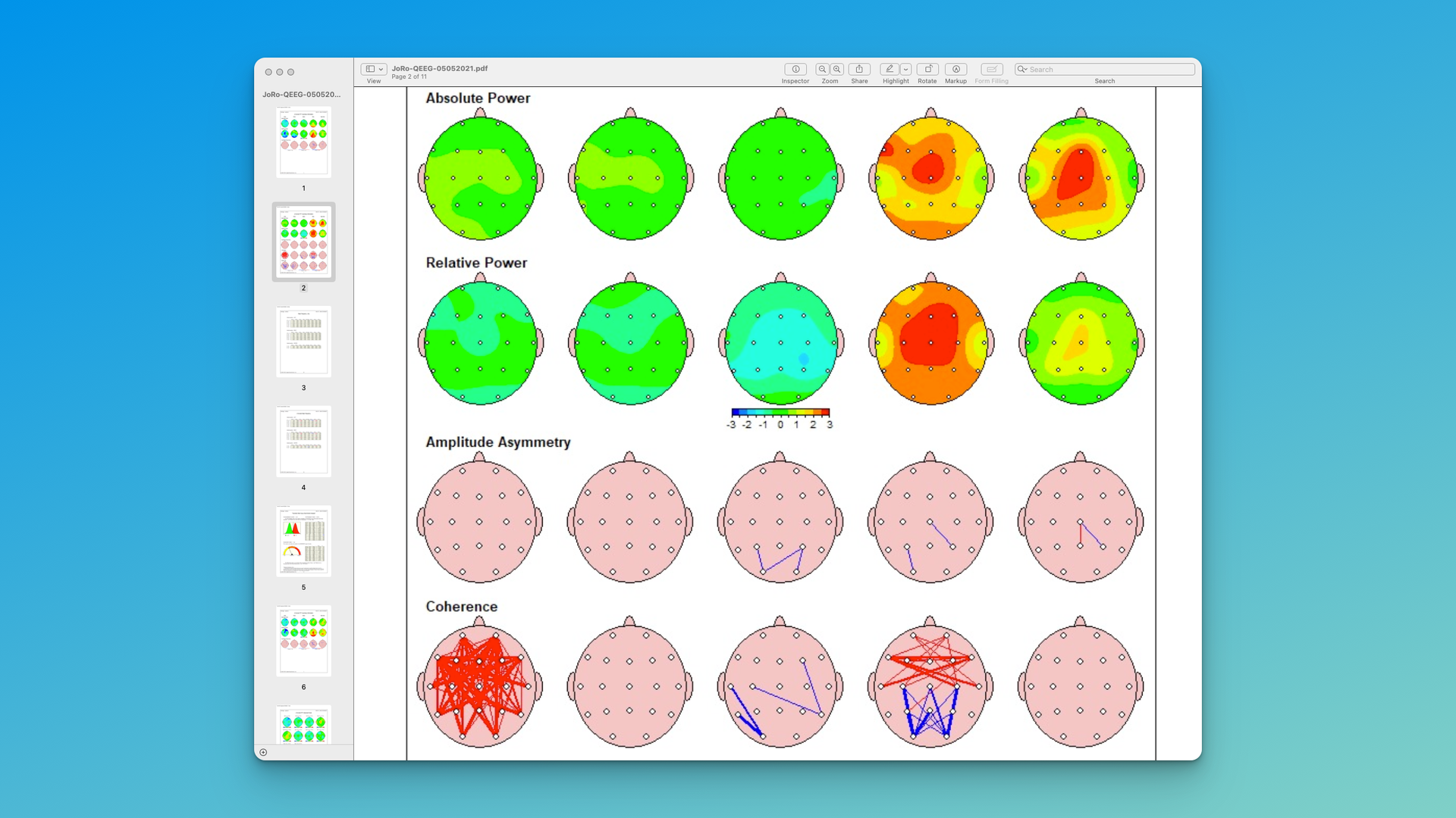Examine raw data as well as 2 montages. For example, you might notice:

• Excess beta activity in the back midline correlating with anxiety issues
• Reduced alpha in the frontal region associated with obsessiveness
• EMG (muscle noise) at front left (F7)

It is crucial to identify the sources of background EEG noise or artifact that might be in the raw data. LORETA will just create false sources if the scalp data is not clean of muscle and other artifact.

Refer to Part 1 of this mini-series on using your own QEEG data, to get tips on working with raw data and QEEG “flat” maps.

Beyond Neurofeedback: How to Use the Z-Qcore QEEG for sLORETA Analysis

Once you’ve identified your areas of interest, you’ll use the raw EEG data (typically in .tdt format) that was used to generate the QEEG analysis to perform a LORETA analysis. Here’s how to proceed:

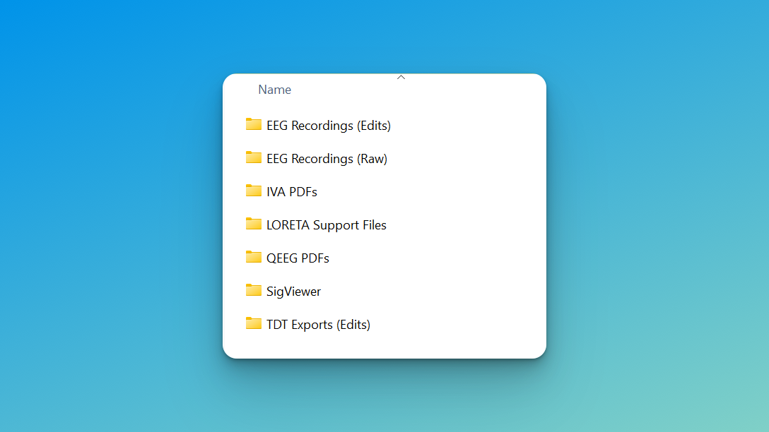
Organizing Your QEEG Data

1. Export Linked Ears EEG files as TDT or CSV files from your recording software, or request those files from your provider.
2. Neuroguide will export as TDT, so we will assume that format for this example. Locate the .tdt files corresponding to the QEEG recording sessions you want to analyze.
3. Create a new folder specifically for this analysis.
4. Copy the relevant .tdt files into this new folder.

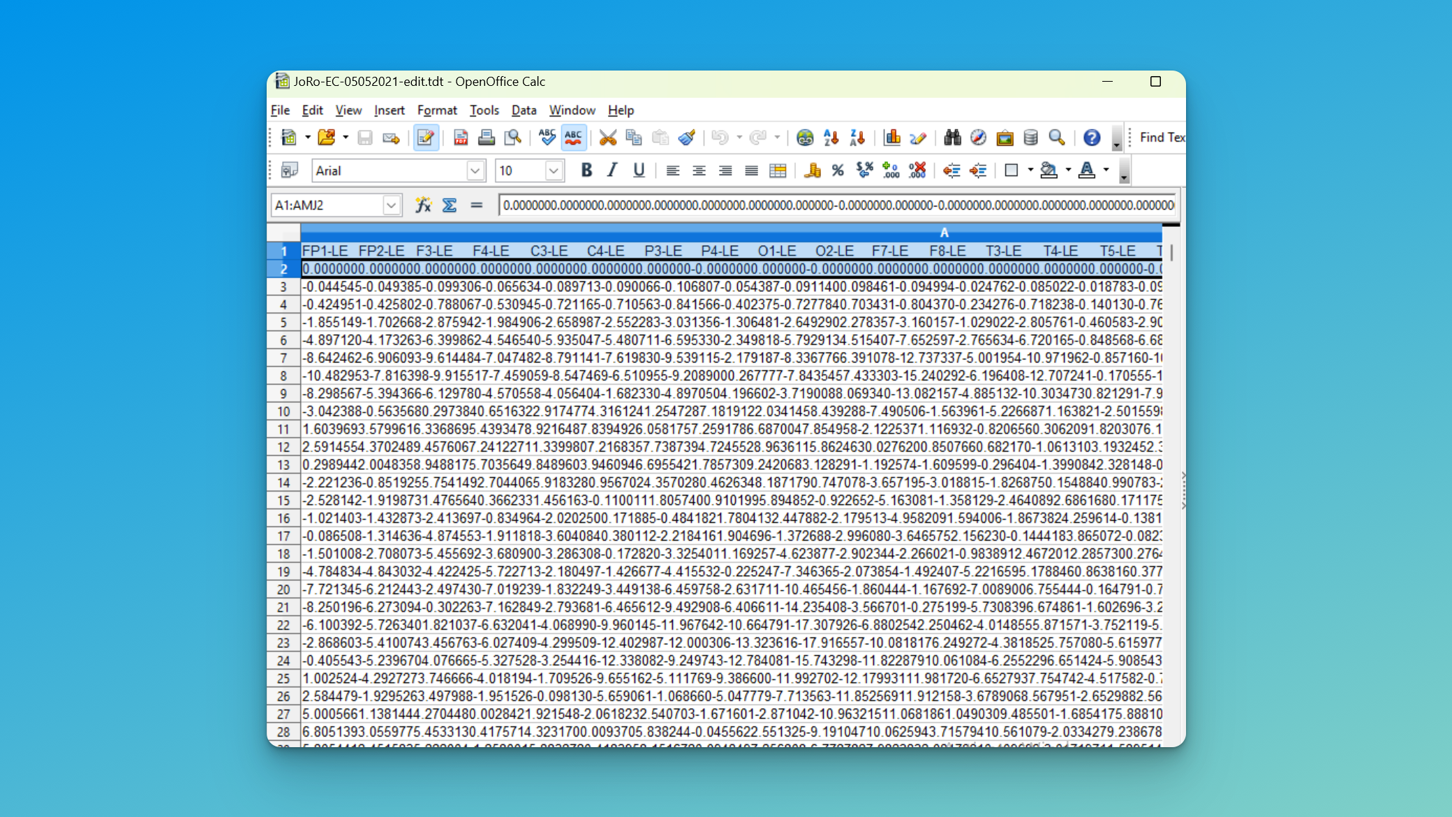
Conversion: How to Use .tdt Files for LORETA 

1. Open each .tdt file in Excel, Google Sheets, or Open Office Calc.
2. Remove the top two rows (electrode placements and zeros).
3. Save each file in .txt format with a descriptive name (e.g., “IDorName_Date_EyesClosed.txt”).

LORETA Data Analysis Workflow: Compute Inverse Solutions (Source Estimation) 

Now, let’s walk through the process of using LORETA to analyze your specific areas of interest. I have collected some files you might need to create the spatial matrix for 19 channel EEG, as well as examples of how to specify the bands you want to look at – you can download the Peak Brain LORETA Support files here.

I. Computational Step 1: Creating Cross Spectra

1. Open LORETA and go to Utilities (top left corner).
2. Select “EEGs to cross spectrum” from the left panel.
3. Choose “Each file to 1 CRS” on the right side.
4. Drag and drop your prepared .txt files into the program.
5. Enter the required information:
   • Number of electrodes: 19 (for standard 10:20 system)
   • Number of time frames per epoch:
     • Double your sampling rate. Example: 500 for Cognionics, 250 for Mitstar, 256 for Neurofield
   • Sampling rate: As per your EEG recording settings
6. Select “User defined bands”.
7. Open the “9 Bands” file from the LoretaSupport folder using Wordpad (not Notepad) or a text editor like vim, to avoid adding other formatting and hidden character line breaks. Edit any bands you want to change, based on what you saw in the EEG and QEEG maps
8. Drag the 9 Bands file into the User defined bands upload section.
9. Click “Go” to convert the files.

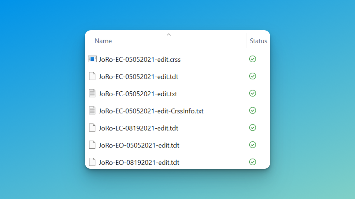
EEG to Cross Spectrum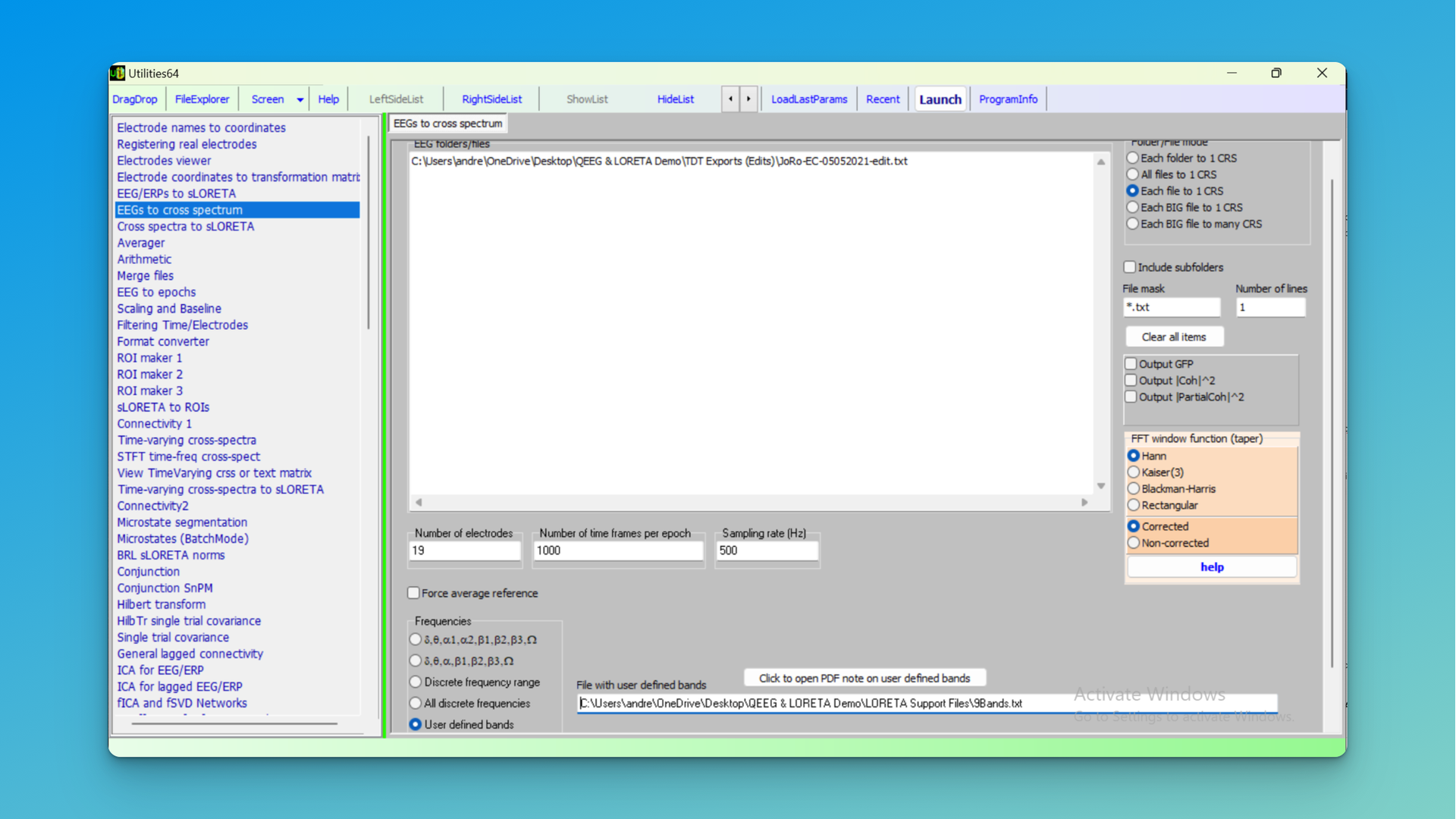

New CRSS files now showing

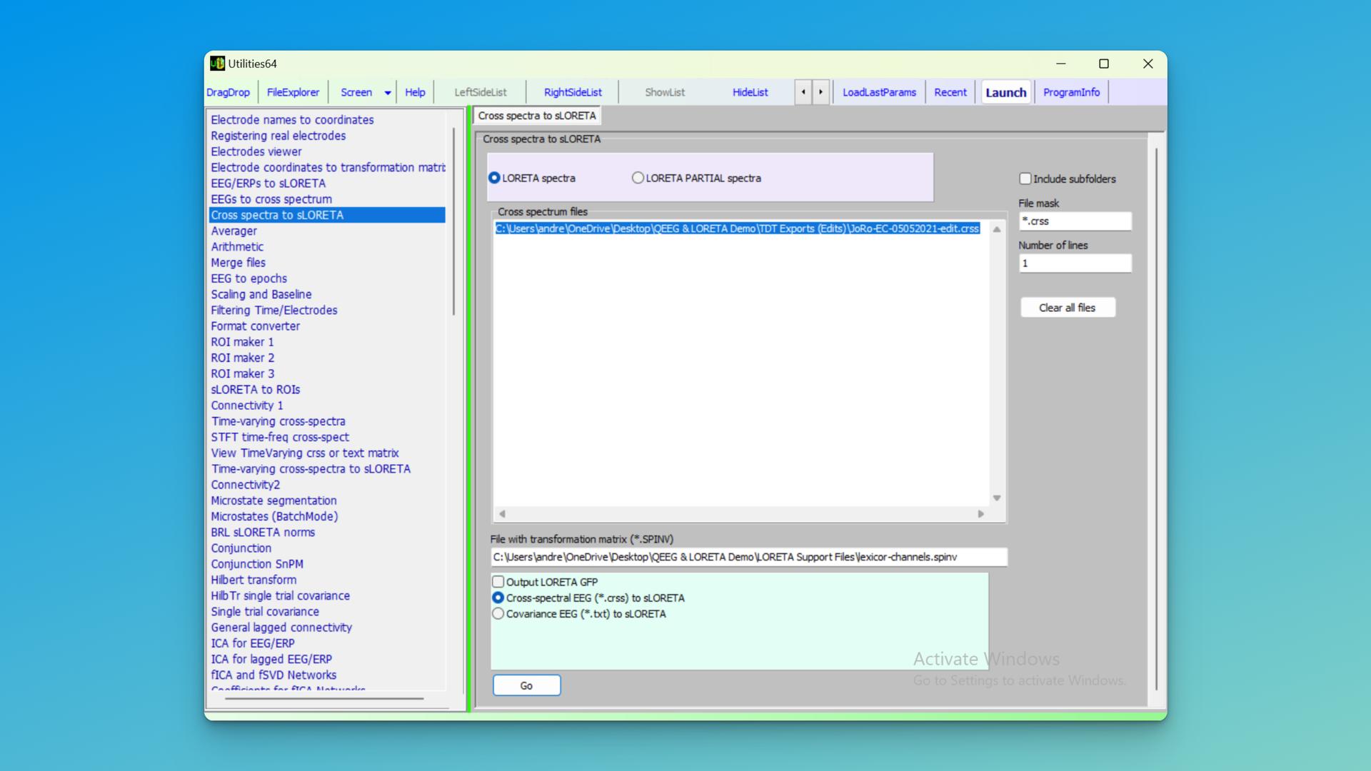
II. Computational Step 2: Converting Cross Spectra to sLORETA

1. In Utilities, select “Cross spectra to sLoreta”.
2. Drag the newly created CRSS files into the white inbox.
3. From the LoretaSupport folder, select or drag the “lexicore.spinv” file into “File with transformation matrix”. This has the XYZ scalp coordinates solved into a matrix.
4. Leave other selections as default, and press Go.
5. New SLOR files will be created in your LoretaAnalysis folder.

III. Visualizing Areas of Brain Function  

1. Close Utilities and open the Viewer from the top menu items in LORETA.
2. Drag an SLOR file into the white inbox.
3. Confirm changing the data to LORETA format.
4. Enter the sampling rate and set the offset to 0.
5. You’ll now see LORETA sources for the 9 bands, although if a large amplitude or wide coverage band, it may be hard to see sources

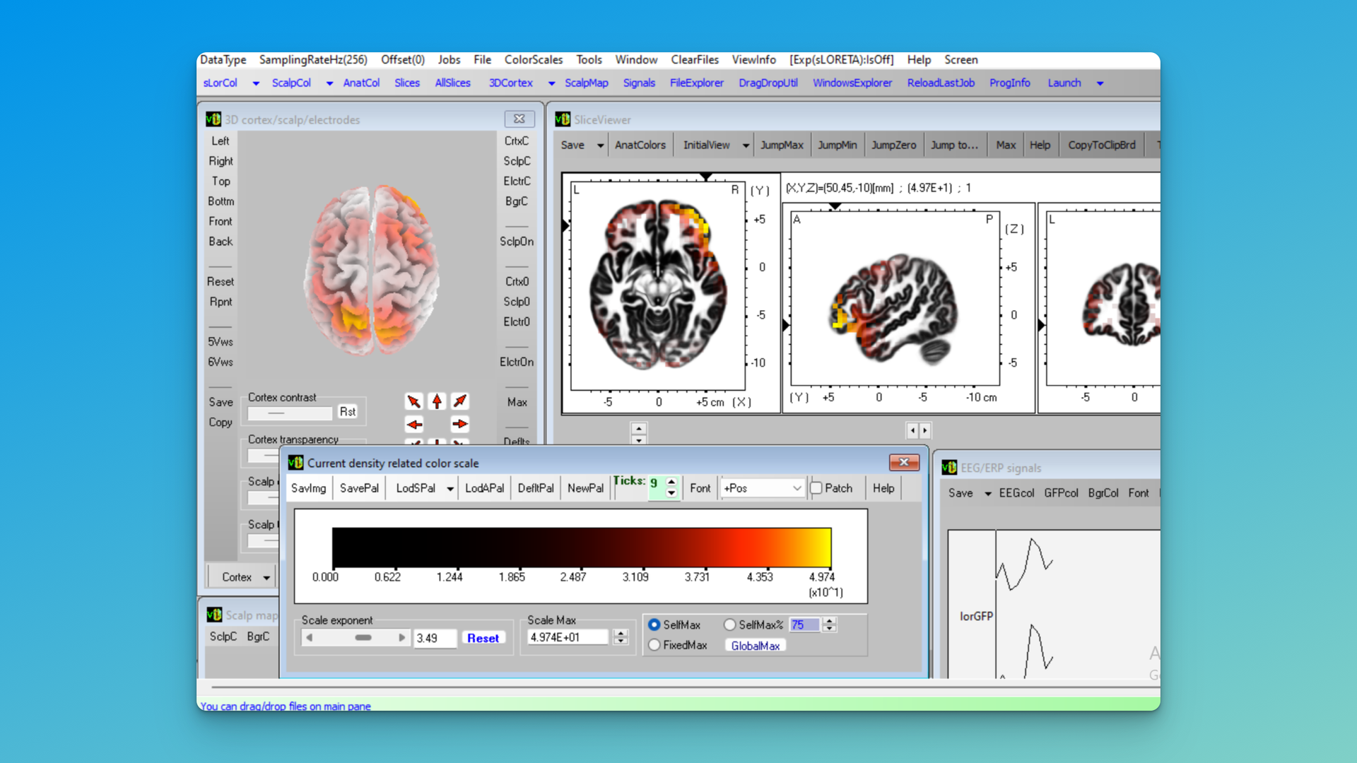
IV. Standardizing Your Analysis

1. Select sLorCol (top left corner).
2. Choose to display positive values only (if desired) or negative, based on waht you are exploring.
3. Adjust the scale to 3.49 (this emphasizes coloring for the top half of the power being generated).
4. Save your scale as “Scale” within the LoretaAnalysis folder for future use.

Unscaled LORETA, Pos and Neg, TF1 (Delta) Selected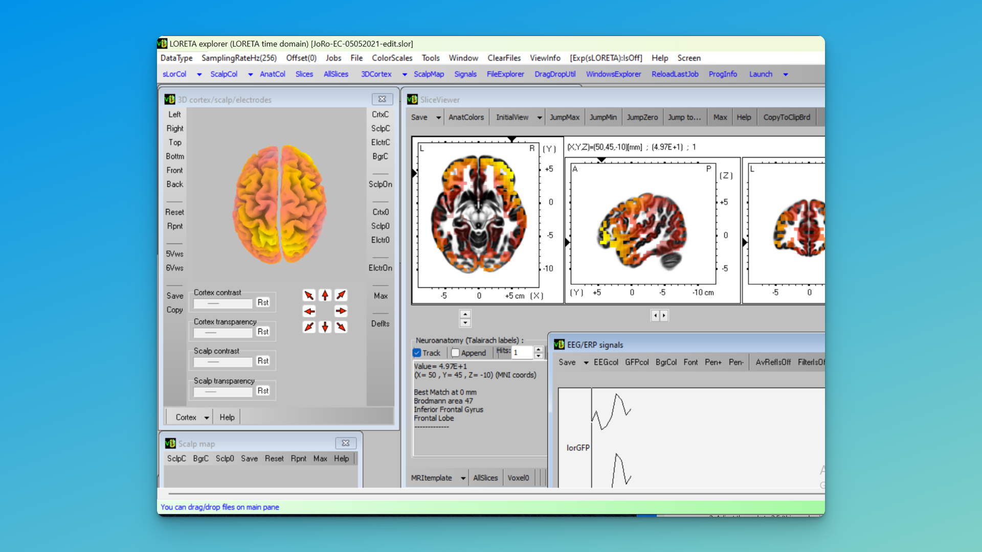Scaled LORETA – TF1 (Delta) Selected

Scaled LORETA – TF6 (Beta 2) Selected

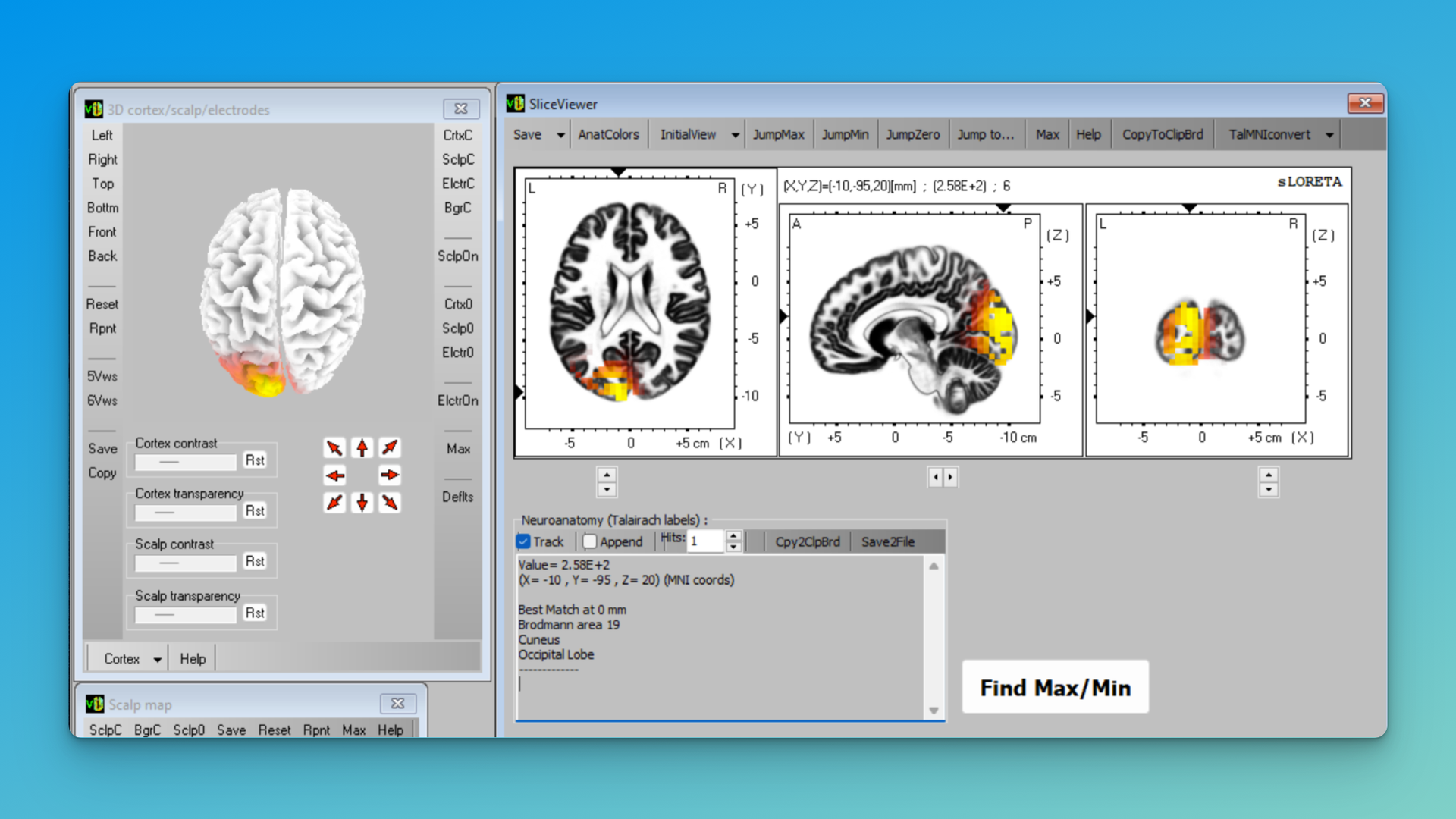
V. Explore Specific Frequencies and Regions

1. Use the EEG/ERP signals table to select the band of interest (see the bottom right label).
   • TF (Time Frame) represents the band: TF = 1 is Delta (2.0-3.5 Hz), etc
2. Use the 5Vw or 6Vw options for multiple brain angles.

By default the Viewer will show you a movable 3D head and the XYZ slice viewer. Select All Slices at the bottom of the Slice Viewer, or 6Vws in the 3D viewer, to see additional visualizations.

All Slices (Beta 2)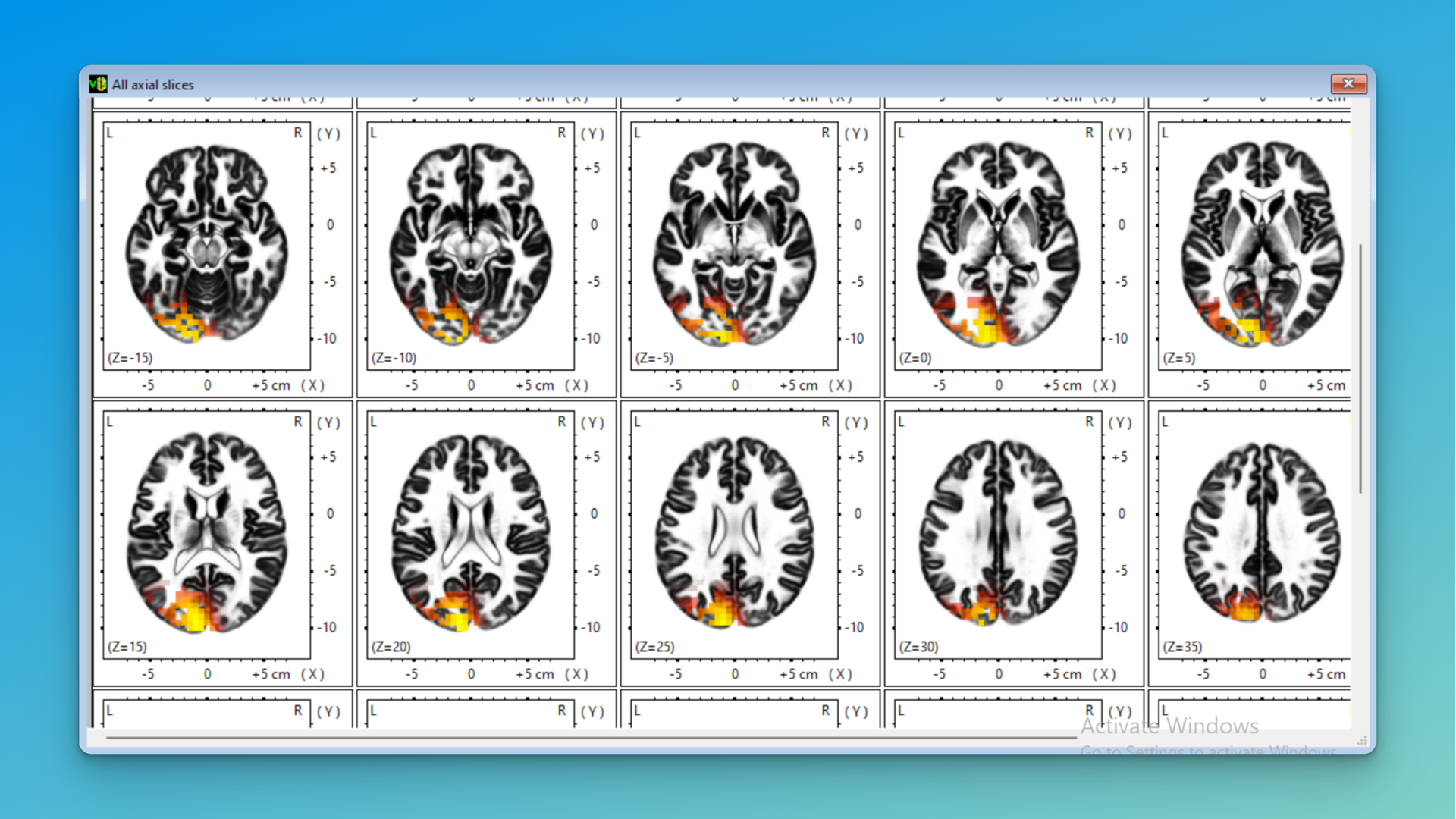

6Vws (Beta 2)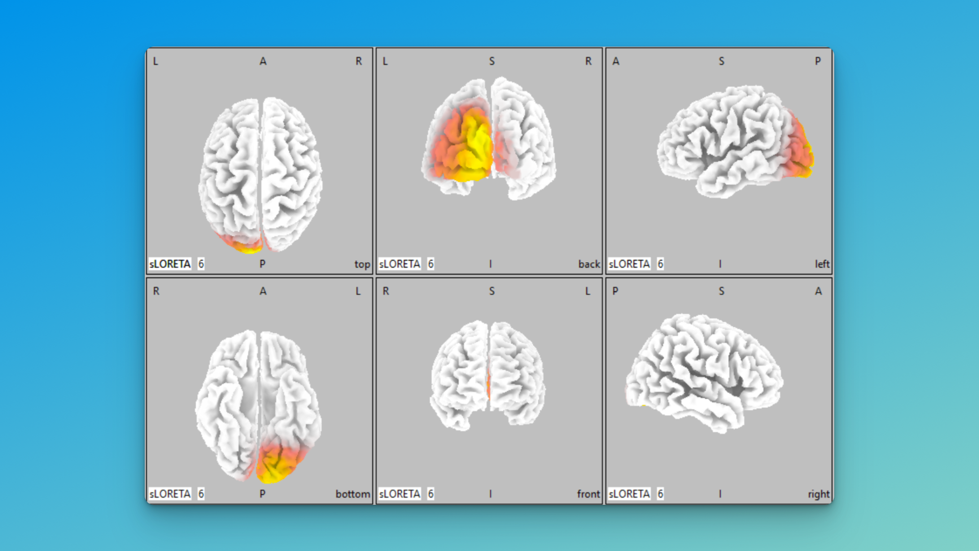

VI. Interpreting Your Results

When examining your 3D LORETA visualizations:

• Compare the activity in your area of interest to surrounding regions.
• Note the intensity and extent of the activity.
• Consider how this 3D view enhances your understanding compared to the flat QEEG maps.
• Reflect on how these findings correlate with the subject’s symptoms or behaviors.

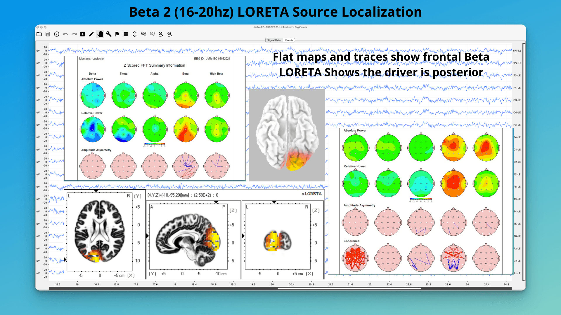
Example: Analyzing Beta Activity

Let’s walk through the specific example above:

1. Initial observation: Flat QEEG maps showed excess beta, at both posterior and frontal midline sites, in different montages. Raw data shows the beta, but also shows a touch of EMG at left front (F7).  Question – where is the beta actually “coming from”?
2. LORETA setup:
   • Prepare the eyes-closed .tdt file, after making sure you have clean data in the frontal region, visually focusing on frontal electrodes (Fp1, Fp2, F3, F4, F7, F8, Fz)
   • Follow the steps above to create SLOR files.
3. Visualization
   • In the LORETA Viewer, select the beta band that corresponds to the 9-bands file (TF6).
   • Focus the view on the frontal lobe, occipital, etc.
   • Observe the intensity and distribution of beta activity.
4. Interpretation:
   • Note areas of peak activity.
   • Compare to normative data or QEEG if available.
   • Consider implications for attention networks and potential interventions.

Where is that Beta coming from?  Back midline.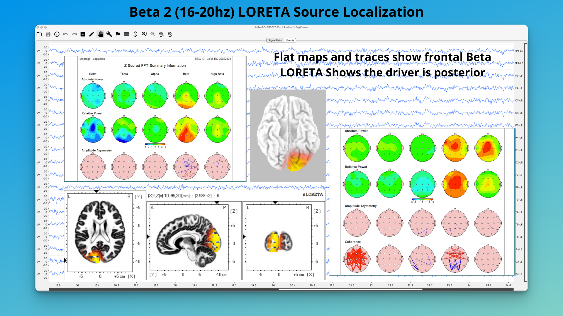

Tutorial Conclusion

By following these steps, you’ve now transformed your initial QEEG observations into detailed 3D visualizations of brain activity. This process allows for a more nuanced understanding of the brain’s electrical patterns, potentially informing more targeted interventions or further areas of investigation.

Remember, while LORETA provides powerful insights, interpretation should always be done in conjunction with clinical findings and under the guidance of qualified professionals. The ability to pinpoint specific frequencies and regions of interest can be invaluable in developing personalized treatment plans or research hypotheses.

Tips and Troubleshooting

• LORETA may crash if you click around too quickly. If this happens, simply restart the program and reopen your generated files.
• Always double-check your sampling rate and electrode count, as these affect the final visualization.
• Use Wordpad instead of Notepad when editing the Bands file to ensure correct formatting.
• Save your work frequently and standardize your analyses for consistent results.

Further Topics: Advanced LORETA Applications and Concepts

As you become more familiar with LORETA, you’ll encounter more advanced concepts and applications. Here are some key areas to explore:

1. Source Localization Techniques

LORETA is part of a family of source localization techniques in EEG analysis. These methods aim to solve the “inverse problem” of identifying the sources of electrical activity measured on the scalp. Other techniques include:

• Minimum Norm Estimates (MNE)
• Beamforming
• Dipole fitting

Each method has its strengths and limitations, with LORETA offering a balance between spatial resolution and computational efficiency.

2. (Low Resolution) Brain Electromagnetic Tomography

LORETA falls under the broader category of Brain Electromagnetic Tomography. This field combines principles from neuroscience, physics, and mathematics to create 3D representations of brain activity from electromagnetic measurements.

3. Quantitative EEG (QEEG) & LORETA Neurofeedback Approaches

While we’ve discussed using LORETA to enhance QEEG analysis, it’s worth noting that LORETA can be fully integrated into QEEG workflows. This integration allows for:

• Z-score analysis in 3D space
• Comparison with normative databases
• Enhanced brain mapping capabilities
• Realtime source analysis neurofeedback may be useful if using full-head caps for training is interesting. Sessions will be slightly shorter than traditional neurofeedback with 3-5 wires at once, but the process will require much more care to get clean cap data each time – any noise in the EEG (from muscle) will distort the LORETA-based neurofeedback process.

4. Functional Connectivity Between Areas of the Brain

LORETA can be used to study functional connectivity in the brain. This involves:

• Analyzing coherence between different brain regions
• Identifying networks of coordinated brain activity
• Studying how these networks change in different recording conditions, across medication, injury, aging, or to explore changes from neurofeeback.

5. Current Source Density (CSD) Source Space

LORETA provides estimates of current source density throughout the brain volume. This allows researchers to:

• Identify areas of high electrical activity
• Study the spread of activity across cortical and subcortical structures
• Compare activity levels in specific brain structures across conditions

6. Time-Domain Analysis

While we’ve focused on frequency-domain analysis, LORETA can also be applied to time-domain EEG data. This allows for:

• Analysis of event-related potentials (ERPs)
• Studying the propagation of activity over time
• Identifying the temporal sequence of activation across brain regions

7. Clinical and Research Applications

LORETA has wide-ranging applications in both clinical practice and neuroscience research:

• Psychiatry: Studying brain activity patterns in conditions like depression, ADHD, and schizophrenia
• Neurology: Localizing seizure foci in epilepsy
• Cognitive Neuroscience: Investigating brain areas involved in specific cognitive processes
• Neurofeedback: Developing targeted protocols based on 3D localization of brain activity

8. Integration with Other Neuroimaging Techniques

LORETA results can be combined with other neuroimaging methods for multimodal analysis:

• fMRI: Comparing hemodynamic responses with electrical activity
• DTI (Diffusion Tensor Imaging): Relating white matter tracts to functional connectivity
• PET: Correlating metabolic activity with electrical patterns

By exploring these advanced concepts and applications, you can leverage the full power of LORETA in your EEG analysis and research endeavors.

Have fun exploring your EEG, with LORETA and beyond, and take care of that brain!